Analysis of ordinal outcome
Analysis methods
1. Proportional odds (PO) model
- Assumptions [1]
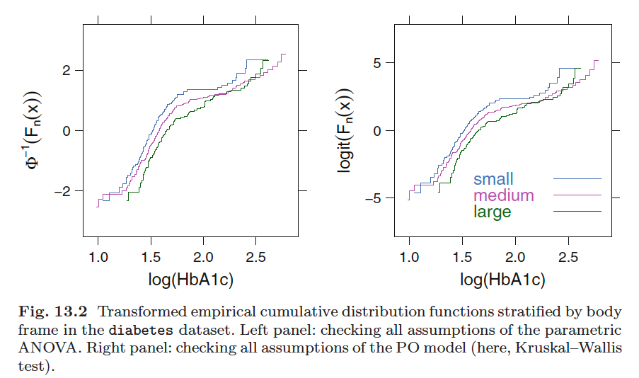
- Parallelism: the logit of the CDFs of different groups should be parallel (equal distance) to each other
- Check this assumption: calculated the empirical CDF(ECDF) for the response variable by group; take logit transformation of the ECDF; check for parallelism
- Linearity: required ONLY if using a parametric logistic distribution instead of semi-parametric PO model
- Parallelism: the logit of the CDFs of different groups should be parallel (equal distance) to each other
- It’s semi-parametric model in the sense that it assumes additivity and linearity (by default) in formulating the probabilities but it doesn’t assume the distribution of the response variable $Y$
- PO model assumes nothing about the actual $Y$ distribution; it only assumes how the distribution of $Y$ for one group is connected to the distribution of another group, i.e. the logit of the cumulative distribution functions are parallel
Connection with Wilcoxon/Kruskal-Wallis test
- PO is also what the Wilcoxon/Kruskal-Wallis test assumes to have optimal power
- By treating all the distinct values in the response variable as a level, then the outcome can be seen as a ordinal variable with many categories
- The hypothesis that the Wilcoxon test possess, i.e. the probability a random sample from group A is greater than a random sample from group B, is technically identical to that the general PO model tries to test (OR = 1 for any cutoff)
- Numerator of the score test for the PO model, when there is only the grouping variable in the model (i.e. not adjusted), is exactly the Wilcoxon statistic
- Kruskal-Wallis test can be formed using a PO model with more than one indicator variable
- This can solve the transivity problem when conducting the pairwise Wilxoson tests [2]
- Model (with 4 groups): $logit[P(Y\ge y|\text{group})] = \alpha_y + \beta_1B + \beta_2C + \beta_3D$
Advantages of PO model vs purely non-parametric counterparts
- can adjust for (continuous) covariates
- more accurate p-values even with extreme number of tied values
- provides a framework for consistent pairwise comparisons [2:1]
- provides estimates of means, quantiles, and exceedance probabilities [3]
- sets the sage for Bayesian PO model, so can get a Bayesian Wilcoxon test
Software
-
rmspackage inRrms::orm(y ~ group)
-
Hmiscpackage inR-
Power calculation with
popowerandposamsize -
simRegOrdfunction can also simulate power for an adjusted two-sample comparisonif there is one adjustment covariate
-
2. Check PO assumption
-
Score test in
PROC LOGISTIC: extreme anti-conservatism in many cases -
Compare means of $X|Y$ with and without assuming PO
-
Stratifying one each predictor and computing the logits of all proportions of the form $Y\ge j, j = \text{1, 2, }\cdots, k$. When proportional odds holds, the difference in logits between different values of $j$ should be the same at all levels of $X$, because the model dictates that $logit(Y\ge j| X) - logit(Y\ge i|X) = \alpha_j - \alpha_i$, for any constant $X$.
-
We check both the consistency of $logit(Y\ge j| X) - logit(Y\ge i|X)$ at different $X$ levels
-
Or we can check the parallelism of $logit(Y\ge j| X) - logit(Y\ge j|X+k)$ for $Y = 1, \cdots, J$
-
3. Method for PO is not met (?)
-
When analyzing ordinal data where PO is not met, the Wilcoxon test may still work OK but it will not be optimal.
-
One way to generate a non-parametric version of OR (called Wilcoxon Mann Whitney Generalized OR [WMW GenOR]) is introduced in [4] and later discussed in [5]. [6] offered a way to eliminate ties and apply Agresti’s formula directly.
- Note: this statistic isn't really an "odds ratio", rather it's an odds per its mathematic definition
-
WMW GenOR test statistic is defined as
$$\hat{\alpha} = \sum_{j>i} p_{1i}p_{2j}/\sum_{j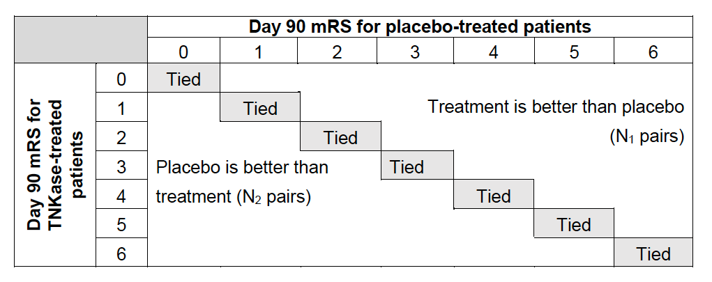
which follows normal distribution with mean $\alpha = Pr(Y_2 > Y_1)/Pr(Y_1 > Y_2)$ and variance
$$\hat{\sigma}^2 = \left\{\frac{1}{N_1}\sum_{j}p_{ij}\left(\hat{\alpha}\sum_{iFurthermore, with patients being stratified into total $M$ strata, the logrithm of test statistic can be written as
$$\log(\hat{\alpha}) = \sum_m^M \hat{\alpha}_m^2 \log\hat{\alpha}_m/\hat{\sigma}_m^2\Bigg/ \sum_{m}^M\hat{\alpha}_m^2/\hat{\sigma}_m^2$$with variance
$$\hat{\sigma}^2 = \left(\sum_m^M\hat{\alpha}_m^2/\hat{\sigma^2_m}\right)^{-1}$$ -
However, I think as long as it uses Wilcoxon type of method, it actually assumes PO in the data
Sample size calculation with ordinal outcome
Method 1: with proportional odds assumption [7]
- Let $Q_{ie\text{ or }c} = \sum_{u=1}^i p_{ue\text{ or }c}, \text{for } i = 1,\cdots, k-1$
- Log odds ratio at cutoff $i$ is defined as $\theta_{iR} = \log\left\{\frac{Q_{ie}(1-Q_{ic})}{(1-Q_{ie})Q_{ic}}\right\}$
- Proportional odds assumption says: $\theta_{iR} = \theta_R = \frac{Q_{e}(1-Q_{c})}{(1-Q_{e})Q_{c}}$ for all $i = 1, \cdots, k-1$
Basic steps
Set up the assumption for outcome distribution
- Assume the percentages at the most commonly used cutoff (e.g. mRS $\le$ 2 vs > 2)
- Based on this assumption, calculate the common odds ratio
- With the assumption of proportional odds, calculate the percentages for each ordinal category and the full distribution of the ordinal outcome can be obtained accordingly
Sample size calculation
using normal approximation
$$n = \frac{3(A+1)^2}{A(1-\sum_{i=1}^k \bar{p}_i^3)}*\frac{(z_{\alpha/2}+z_{\beta})^2}{\theta_R^2},$$where
- $A = n_c/n_e$, is the randomization ratio between control and treated arms
- $\theta_R$ is the log of the common odds ratio for treated vs control arm
- $z_{\alpha/2} = \Phi^{-1}(1-\alpha/2), z_{\beta} = \Phi^{-1}(1-\beta)$
- $\bar{p}_i = \frac{p_{ie} + p_{ic}}{2}$ for $i= 1, \cdots, k$
Method 2: without PO assumtion [8]
Link to notes.
Method 3: without PO assumption [9]
- Exact variance method for the size and power calculation for theWilcoxon–Mann–Whitney test for ordered categorical data.
- Notes to be done
Resources for Ordinal Regression Models
General references
- https://hbiostat.org/bib/ordinal.html which includes tutorials such as the one by Susan Scott et al.
References
t-test assumes both linearity (normal distribution) and parallelism (equal variance) ↩︎
that is, the order of the same observation may be different in different pairwise comparisons, in which different subsets of the data are used. ↩︎ ↩︎
to calculate mean, first calculate the probability of the outcome equals to a specific value, then apply the definition of mean for discrete R.V.: $\bar{X} = \sum_{i} x\cdot Pr(X=x)$; finding median/a specific quantile is simpler, which is a direct result from the cumulative distribution of the outcome variable. ↩︎
Agresti, Alan (1980). Generalized odds ratios for ordinal data. ↩︎
Churilov, Leonid and Arnup, Sarah and Johns, Hayden and Leung, Tiffany and Roberts, Stuart and Campbell, Bruce CV and Davis, Stephen M and Donnan, Geoffrey A (2014). An improved method for simple, assumption-free ordinal analysis of the modified Rankin Scale using generalized odds ratios. ↩︎
O’Brien, Ralph G and Castelloe, John (2006). Exploiting the link between the Wilcoxon-Mann-Whitney test and a simple odds statistic. ↩︎
Whitehead, John (1993). Sample size calculations for ordered categorical data. ↩︎
Zhao, Yan D and Rahardja, Dewi and Qu, Yongming (2008). Sample size calculation for the Wilcoxon--Mann--Whitney test adjusting for ties. ↩︎
Tang, Yongqiang (2011). Size and power estimation for the Wilcoxon--Mann--Whitney test for ordered categorical data. ↩︎